Working with Datasets and Describing Them With Numbers
ISI-BUDS 2025
Getting to Know Data Frames
Data Frame
Data Frame
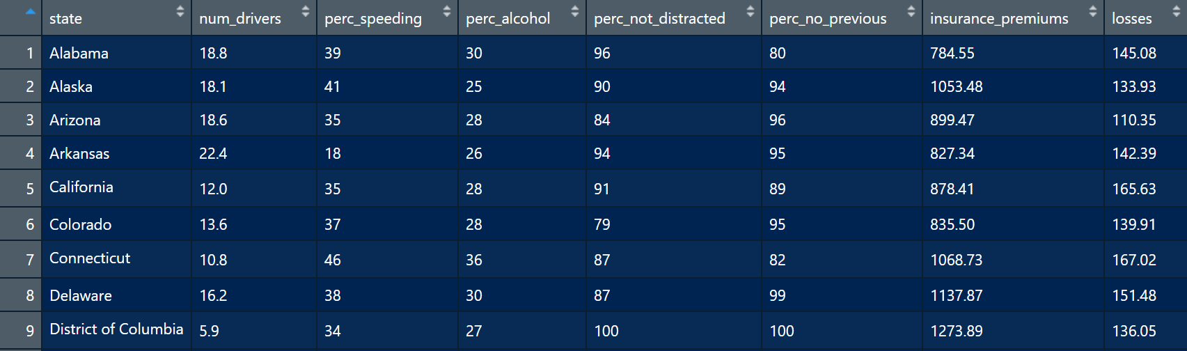
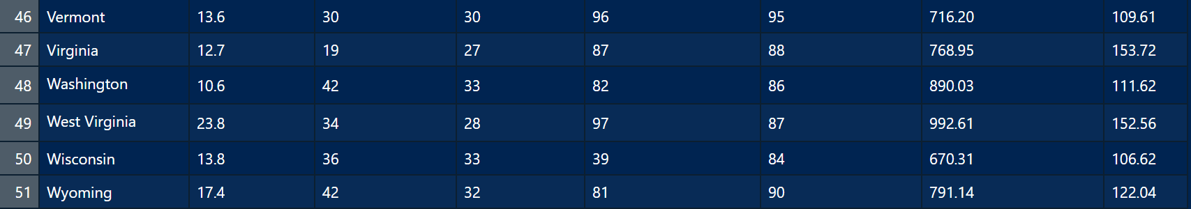
The data frame has 8 variables (state, num_drivers, perc_speeding, perc_not_distracted, perc_no_previous, insurance_premiums, losses).
The data frame has 51 cases or observations. Each case represents a US state (or District of Columbia).
Data documentation
state State
num_drivers Number of drivers involved in fatal collisions per billion miles
perc_speeding Percentage of drivers involved in fatal collisions who were speeding
perc_alcohol Percentage of drivers involved in fatal collisions who were alcohol-impaired
perc_not_distracted Percentage of drivers involved in fatal collisions who were not distracted
perc_no_previous Percentage of drivers involved in fatal collisions who had not been involved in any previous accidents
insurance_premiums Car insurance premiums ($)
losses Losses incurred by insurance companies for collisions per insured driver ($)
Source National Highway Traffic Safety Administration 2012, National Highway Traffic Safety Administration 2009 & 2012, National Association of Insurance Commissioners 2010 & 2011.
# A tibble: 6 × 8
  state      num_drivers perc_speeding perc_alcohol perc_not_distracted
  <chr>            <dbl>         <int>        <int>               <int>
1 Alabama           18.8            39           30                  96
2 Alaska            18.1            41           25                  90
3 Arizona           18.6            35           28                  84
4 Arkansas          22.4            18           26                  94
5 California        12              35           28                  91
6 Colorado          13.6            37           28                  79
# ℹ 3 more variables: perc_no_previous <int>, insurance_premiums <dbl>,
# losses <dbl># A tibble: 6 × 8
state num_drivers perc_speeding perc_alcohol perc_not_distracted
<chr> <dbl> <int> <int> <int>
1 Vermont 13.6 30 30 96
2 Virginia 12.7 19 27 87
3 Washington 10.6 42 33 82
4 West Virginia 23.8 34 28 97
5 Wisconsin 13.8 36 33 39
6 Wyoming 17.4 42 32 81
# ℹ 3 more variables: perc_no_previous <int>, insurance_premiums <dbl>,
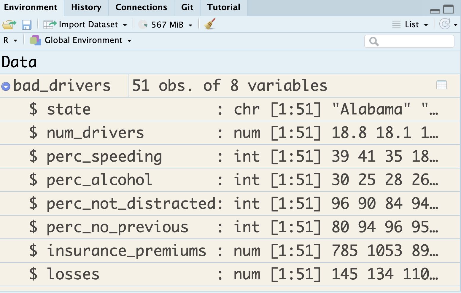
# losses <dbl>Rows: 51
Columns: 8
$ state <chr> "Alabama", "Alaska", "Arizona", "Arkansas", "Calif…
$ num_drivers <dbl> 18.8, 18.1, 18.6, 22.4, 12.0, 13.6, 10.8, 16.2, 5.…
$ perc_speeding <int> 39, 41, 35, 18, 35, 37, 46, 38, 34, 21, 19, 54, 36…
$ perc_alcohol <int> 30, 25, 28, 26, 28, 28, 36, 30, 27, 29, 25, 41, 29…
$ perc_not_distracted <int> 96, 90, 84, 94, 91, 79, 87, 87, 100, 92, 95, 82, 8…
$ perc_no_previous <int> 80, 94, 96, 95, 89, 95, 82, 99, 100, 94, 93, 87, 9…
$ insurance_premiums <dbl> 784.55, 1053.48, 899.47, 827.34, 878.41, 835.50, 1…
$ losses <dbl> 145.08, 133.93, 110.35, 142.39, 165.63, 139.91, 16…Getting to Know the Data Frame
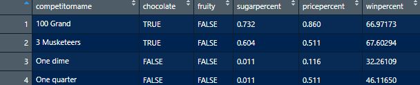
Rows: 85
Columns: 6
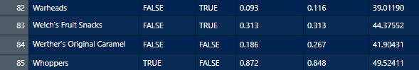
$ competitorname <chr> "100 Grand", "3 Musketeers", "One dime", "One quarter",…
$ chocolate <lgl> TRUE, TRUE, FALSE, FALSE, FALSE, TRUE, TRUE, FALSE, FAL…
$ fruity <lgl> FALSE, FALSE, FALSE, FALSE, TRUE, FALSE, FALSE, FALSE, …
$ sugarpercent <dbl> 0.732, 0.604, 0.011, 0.011, 0.906, 0.465, 0.604, 0.313,…
$ pricepercent <dbl> 0.860, 0.511, 0.116, 0.511, 0.511, 0.767, 0.767, 0.511,…
$ winpercent <dbl> 66.97173, 67.60294, 32.26109, 46.11650, 52.34146, 50.34…Rows: 403
Columns: 71
$ episode <chr> "S01E01", "S01E02", "S01E03", "S01E04", "S01E05", "…
$ season <dbl> 1, 1, 1, 1, 1, 1, 1, 1, 1, 1, 1, 1, 1, 2, 2, 2, 2, …
$ episode_num <dbl> 1, 2, 3, 4, 5, 6, 7, 8, 9, 10, 11, 12, 13, 1, 2, 3,…
$ title <chr> "A WALK IN THE WOODS", "MT. MCKINLEY", "EBONY SUNSE…
$ apple_frame <int> 0, 0, 0, 0, 0, 0, 0, 0, 0, 0, 0, 0, 0, 0, 0, 0, 0, …
$ aurora_borealis <int> 0, 0, 0, 0, 0, 0, 0, 0, 0, 0, 0, 0, 0, 0, 0, 0, 0, …
$ barn <int> 0, 0, 0, 0, 0, 0, 0, 0, 0, 0, 0, 0, 0, 0, 0, 0, 0, …
$ beach <int> 0, 0, 0, 0, 0, 0, 0, 0, 1, 0, 0, 0, 0, 0, 0, 0, 0, …
$ boat <int> 0, 0, 0, 0, 0, 0, 0, 0, 0, 0, 0, 0, 0, 0, 0, 0, 0, …
$ bridge <int> 0, 0, 0, 0, 0, 0, 0, 0, 0, 0, 0, 0, 0, 0, 0, 0, 0, …
$ building <int> 0, 0, 0, 0, 0, 0, 0, 0, 0, 0, 0, 0, 0, 0, 0, 0, 0, …
$ bushes <int> 1, 0, 0, 1, 0, 0, 0, 1, 0, 1, 0, 0, 1, 1, 0, 0, 1, …
$ cabin <int> 0, 1, 1, 0, 0, 1, 0, 0, 0, 0, 0, 0, 0, 0, 0, 0, 1, …
$ cactus <int> 0, 0, 0, 0, 0, 0, 0, 0, 0, 0, 0, 0, 0, 0, 0, 0, 0, …
$ circle_frame <int> 0, 0, 0, 0, 0, 0, 0, 0, 0, 0, 0, 0, 0, 0, 0, 0, 0, …
$ cirrus <int> 0, 0, 0, 0, 0, 0, 0, 0, 0, 0, 0, 1, 0, 0, 0, 0, 0, …
$ cliff <int> 0, 0, 0, 0, 0, 0, 0, 0, 0, 0, 0, 0, 0, 0, 0, 0, 0, …
$ clouds <int> 0, 1, 0, 1, 0, 0, 0, 0, 1, 0, 0, 1, 0, 0, 0, 1, 1, …
$ conifer <int> 0, 1, 1, 1, 0, 1, 0, 1, 0, 1, 0, 1, 1, 1, 1, 0, 1, …
$ cumulus <int> 0, 0, 0, 0, 0, 0, 0, 0, 0, 0, 0, 0, 0, 1, 0, 1, 1, …
$ deciduous <int> 1, 0, 0, 0, 1, 0, 1, 0, 0, 1, 1, 0, 1, 1, 0, 1, 1, …
$ diane_andre <int> 0, 0, 0, 0, 0, 0, 0, 0, 0, 0, 0, 0, 0, 0, 0, 0, 0, …
$ dock <int> 0, 0, 0, 0, 0, 0, 0, 0, 0, 0, 0, 0, 0, 0, 0, 0, 0, …
$ double_oval_frame <int> 0, 0, 0, 0, 0, 0, 0, 0, 0, 0, 0, 0, 0, 0, 0, 0, 0, …
$ farm <int> 0, 0, 0, 0, 0, 0, 0, 0, 0, 0, 0, 0, 0, 0, 0, 0, 0, …
$ fence <int> 0, 0, 1, 0, 0, 0, 0, 0, 1, 0, 0, 0, 0, 0, 0, 0, 0, …
$ fire <int> 0, 0, 0, 0, 0, 0, 0, 0, 0, 0, 0, 0, 0, 0, 0, 0, 0, …
$ florida_frame <int> 0, 0, 0, 0, 0, 0, 0, 0, 0, 0, 0, 0, 0, 0, 0, 0, 0, …
$ flowers <int> 0, 0, 0, 0, 0, 0, 0, 0, 0, 0, 0, 0, 0, 0, 0, 0, 0, …
$ fog <int> 0, 0, 0, 0, 0, 0, 0, 0, 0, 0, 0, 0, 0, 0, 0, 0, 0, …
$ framed <int> 0, 0, 0, 0, 0, 0, 0, 0, 0, 0, 0, 0, 0, 0, 0, 0, 0, …
$ grass <int> 1, 0, 0, 0, 0, 0, 0, 0, 0, 0, 0, 0, 1, 1, 0, 0, 0, …
$ guest <int> 0, 0, 0, 0, 0, 0, 0, 0, 0, 0, 0, 0, 0, 0, 0, 0, 0, …
$ half_circle_frame <int> 0, 0, 0, 0, 0, 0, 0, 0, 0, 0, 0, 0, 0, 0, 0, 0, 0, …
$ half_oval_frame <int> 0, 0, 0, 0, 0, 0, 0, 0, 0, 0, 0, 0, 0, 0, 0, 0, 0, …
$ hills <int> 0, 0, 0, 0, 0, 0, 0, 0, 0, 0, 0, 0, 0, 0, 0, 0, 0, …
$ lake <int> 0, 0, 0, 1, 0, 1, 1, 1, 0, 1, 1, 1, 0, 1, 1, 0, 1, …
$ lakes <int> 0, 0, 0, 0, 0, 0, 0, 0, 0, 0, 0, 0, 0, 0, 0, 0, 0, …
$ lighthouse <int> 0, 0, 0, 0, 0, 0, 0, 0, 0, 0, 0, 0, 0, 0, 0, 0, 0, …
$ mill <int> 0, 0, 0, 0, 0, 0, 0, 0, 0, 0, 0, 0, 0, 0, 0, 0, 0, …
$ moon <int> 0, 0, 0, 0, 0, 1, 0, 0, 0, 0, 0, 0, 0, 0, 0, 0, 0, …
$ mountain <int> 0, 1, 1, 1, 0, 1, 1, 1, 0, 1, 0, 1, 1, 1, 0, 0, 1, …
$ mountains <int> 0, 0, 1, 0, 0, 1, 1, 1, 0, 0, 0, 1, 0, 0, 0, 0, 1, …
$ night <int> 0, 0, 0, 0, 0, 1, 0, 0, 0, 0, 0, 0, 0, 0, 0, 0, 0, …
$ ocean <int> 0, 0, 0, 0, 0, 0, 0, 0, 1, 0, 0, 0, 0, 0, 0, 1, 0, …
$ oval_frame <int> 0, 0, 0, 0, 0, 0, 0, 0, 0, 0, 0, 0, 0, 0, 0, 0, 0, …
$ palm_trees <int> 0, 0, 0, 0, 0, 0, 0, 0, 0, 0, 0, 0, 0, 0, 0, 0, 0, …
$ path <int> 0, 0, 0, 0, 0, 0, 0, 0, 0, 0, 0, 0, 0, 0, 0, 0, 0, …
$ person <int> 0, 0, 0, 0, 0, 0, 0, 0, 0, 0, 0, 0, 0, 0, 0, 0, 0, …
$ portrait <int> 0, 0, 0, 0, 0, 0, 0, 0, 0, 0, 0, 0, 0, 0, 0, 0, 0, …
$ rectangle_3d_frame <int> 0, 0, 0, 0, 0, 0, 0, 0, 0, 0, 0, 0, 0, 0, 0, 0, 0, …
$ rectangular_frame <int> 0, 0, 0, 0, 0, 0, 0, 0, 0, 0, 0, 0, 0, 0, 0, 0, 0, …
$ river <int> 1, 0, 0, 0, 1, 0, 0, 0, 0, 0, 0, 0, 0, 0, 0, 0, 0, …
$ rocks <int> 0, 0, 0, 0, 1, 0, 0, 0, 0, 0, 0, 0, 0, 0, 0, 0, 0, …
$ seashell_frame <int> 0, 0, 0, 0, 0, 0, 0, 0, 0, 0, 0, 0, 0, 0, 0, 0, 0, …
$ snow <int> 0, 1, 0, 0, 0, 1, 0, 0, 0, 0, 0, 0, 0, 0, 1, 0, 1, …
$ snowy_mountain <int> 0, 1, 0, 1, 0, 1, 1, 0, 0, 0, 0, 1, 1, 1, 0, 0, 1, …
$ split_frame <int> 0, 0, 0, 0, 0, 0, 0, 0, 0, 0, 0, 0, 0, 0, 0, 0, 0, …
$ steve_ross <int> 0, 0, 0, 0, 0, 0, 0, 0, 0, 0, 0, 0, 0, 0, 0, 0, 0, …
$ structure <int> 0, 0, 1, 0, 0, 1, 0, 0, 0, 0, 0, 0, 0, 0, 0, 0, 1, …
$ sun <int> 0, 0, 1, 0, 0, 0, 0, 0, 0, 0, 0, 0, 0, 0, 1, 1, 0, …
$ tomb_frame <int> 0, 0, 0, 0, 0, 0, 0, 0, 0, 0, 0, 0, 0, 0, 0, 0, 0, …
$ tree <int> 1, 1, 1, 1, 1, 1, 1, 1, 0, 1, 1, 1, 1, 1, 1, 1, 1, …
$ trees <int> 1, 1, 1, 1, 1, 1, 1, 1, 0, 1, 1, 1, 1, 1, 1, 1, 1, …
$ triple_frame <int> 0, 0, 0, 0, 0, 0, 0, 0, 0, 0, 0, 0, 0, 0, 0, 0, 0, …
$ waterfall <int> 0, 0, 0, 0, 0, 0, 0, 0, 0, 0, 0, 0, 0, 0, 0, 0, 0, …
$ waves <int> 0, 0, 0, 0, 0, 0, 0, 0, 0, 0, 0, 0, 0, 0, 0, 1, 0, …
$ windmill <int> 0, 0, 0, 0, 0, 0, 0, 0, 0, 0, 0, 0, 0, 0, 0, 0, 0, …
$ window_frame <int> 0, 0, 0, 0, 0, 0, 0, 0, 0, 0, 0, 0, 0, 0, 0, 0, 0, …
$ winter <int> 0, 1, 1, 0, 0, 1, 0, 0, 0, 0, 0, 0, 0, 0, 0, 0, 0, …
$ wood_framed <int> 0, 0, 0, 0, 0, 0, 0, 0, 0, 0, 0, 0, 0, 0, 0, 0, 0, …Rows: 143
Columns: 12
$ id <dbl> 150377422259, 260483376854, 320432342985, 280405224677, 17…
$ duration <int> 3, 7, 3, 3, 1, 3, 1, 1, 3, 7, 1, 1, 1, 1, 7, 7, 3, 3, 1, 7…
$ n_bids <int> 20, 13, 16, 18, 20, 19, 13, 15, 29, 8, 15, 15, 13, 16, 6, …
$ cond <fct> new, used, new, new, new, new, used, new, used, used, new,…
$ start_pr <dbl> 0.99, 0.99, 0.99, 0.99, 0.01, 0.99, 0.01, 1.00, 0.99, 19.9…
$ ship_pr <dbl> 4.00, 3.99, 3.50, 0.00, 0.00, 4.00, 0.00, 2.99, 4.00, 4.00…
$ total_pr <dbl> 51.55, 37.04, 45.50, 44.00, 71.00, 45.00, 37.02, 53.99, 47…
$ ship_sp <fct> standard, firstClass, firstClass, standard, media, standar…
$ seller_rate <int> 1580, 365, 998, 7, 820, 270144, 7284, 4858, 27, 201, 4858,…
$ stock_photo <fct> yes, yes, no, yes, yes, yes, yes, yes, yes, no, yes, yes, …
$ wheels <int> 1, 1, 1, 1, 2, 0, 0, 2, 1, 1, 2, 2, 2, 2, 1, 0, 1, 1, 2, 2…
$ title <fct> "~~ Wii MARIO KART & WHEEL ~ NINTENDO Wii ~ BRAND NEW …Variables
In Statistics
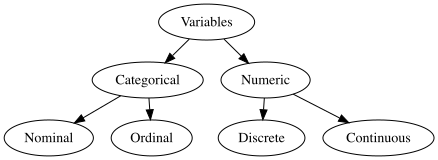
(Some) Variable Types in R
character: takes string values (e.g. a person’s name, address)
integer: integer (single precision)
double: floating decimal (double precision)
numeric: integer or double
factor: categorical variables with different levels
logical: TRUE (1), FALSE (0)
As a data scientist it is your job to check the type(s) of data that you are working with. Do not assume you will work with clean data frames, with clean names, labels, and types.
Describing Data with Numbers
Data
Rows: 75
Columns: 3
$ group  <fct> control, control, control, control, control, control, control, …
$ years  <int> 0, 0, 0, 0, 0, 0, 0, 0, 0, 0, 0, 0, 0, 0, 0, 0, 0, 0, 0, 0, 0, …
$ volume <dbl> 6.175, 6.220, 6.360, 6.465, 6.540, 6.780, 6.980, 7.075, 7.120, …
Data
Rows: 75
Columns: 2
$ volume <dbl> 6.175, 6.220, 6.360, 6.465, 6.540, 6.780, 6.980, 7.075, 7.120, …
$ group  <fct> control, control, control, control, control, control, control, …
What kind of variables are these two?
Categorical data are summarized with counts or proportions
Summarizing Numerical Data
Mean
Median
Minimum
In a similar fashion maxiumum can be found by using the max() function.
Standard deviation
Variance
Quantiles / Percentiles / Quartiles
| Quantile | Percentile | Special Name |
|---|---|---|
| 0.25 | 25th | First quartile |
| 0.5 | 50th | Median |
| 0.75 | 75th | Third quartile |
Quantiles
We can get multiple summaries with one summarize() function.
Note how the variables names in this table is not easy to read.
In order to display the variable names more legibly in the output, we can assign variable names to numerical summaries (e.g. mean_volume).
Importing Data
So far we have used data that were part of R packages. What if we wanted to download a dataset online?
Importing .csv Data
Importing Excel Data
Importing Excel Data
Importing SAS, SPSS, Stata Data
Where is the dataset file?
Importing data will depend on where the dataset is on your computer. However we use the help of here::here() function. This function sets the working directory to the project folder (i.e. where the .Rproj file is).
Practice
Download and import
Restaurant and Market Health Inspections from City of LA.
- HIV Antibody Test Note that the data is in XPT format.