Data Wrangling
Part I

ISI-BUDS 2025

Three solutions to a single problem

What is the average of 4, 8, 16 approximately?

1.What is the average of 4, 8, 16 approximately?

2.What is the average of 4, 8, 16 approximately?

3.What is the average of 4, 8, 16 approximately?

Solution 1: Functions within Functions

c(4, 8, 16)

[1]  4  8 16

---

mean(c(4, 8, 16))

[1] 9.333333

---

round(mean(c(4, 8, 16)))

[1] 9

Problem with writing functions within functions

Things will get messy and more difficult to read and debug as we deal with more complex operations on data.

Solution 2: Creating Objects

numbers <- c(4, 8, 16)
numbers

[1]  4  8 16

---

avg_number <- mean(numbers)
avg_number

[1] 9.333333

---

round(avg_number)

[1] 9

Problem with creating many objects

We will end up with too many objects in Environment.

Solution 3: The (forward) Pipe Operator |>

Shortcut:
Ctrl (Command) + Shift + M

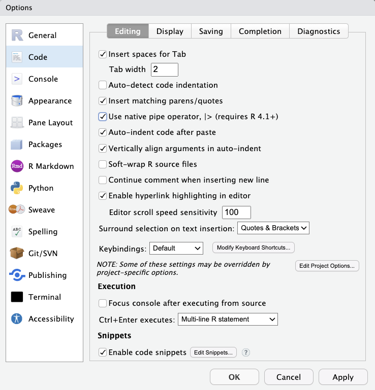
Make sure to select Use native pipe operator under Tools > Global Options > Code

c(4, 8, 16) |> 
  mean() |> 
  round()

[1] 9

Combine 4, 8, and 16 and then
Take the mean and then
Round the output

The output of the first function is the first argument of the second function.

Now we have \(f \circ g \circ h (x)\)
or round(mean(c(4, 8, 16)))

h(x) |> 
  g() |> 
  f()

c(4, 8, 16) |> 
  mean() |> 
  round()

Data

glimpse(covid_data)

Rows: 15,524
Columns: 17
$ subject_id      <dbl> 1412, 533, 9134, 8518, 8967, 11048, 663, 2158, 3794, 4…
$ fake_first_name <chr> "jhezane", "penny", "grunt", "melisandre", "rolley", "…
$ fake_last_name  <chr> "westerling", "targaryen", "rivers", "swyft", "karstar…
$ gender          <chr> "female", "female", "male", "female", "male", "female"…
$ pan_day         <dbl> 4, 7, 7, 8, 8, 8, 9, 9, 9, 9, 9, 9, 9, 9, 9, 10, 10, 1…
$ test_id         <chr> "covid", "covid", "covid", "covid", "covid", "covid", …
$ clinic_name     <chr> "inpatient ward a", "clinical lab", "clinical lab", "c…
$ result          <chr> "negative", "negative", "negative", "negative", "negat…
$ demo_group      <chr> "patient", "patient", "patient", "patient", "patient",…
$ age             <dbl> 0.0, 0.0, 0.8, 0.8, 0.8, 0.8, 0.8, 0.0, 0.0, 0.9, 0.9,…
$ drive_thru_ind  <dbl> 0, 1, 1, 1, 0, 0, 1, 0, 1, 1, 1, 0, 0, 1, 1, 1, 1, 0, …
$ ct_result       <dbl> 45, 45, 45, 45, 45, 45, 45, 45, 45, 45, 45, 45, 45, 45…
$ orderset        <dbl> 0, 0, 1, 1, 1, 0, 1, 1, 1, 1, 0, 1, 0, 1, 1, 1, 1, 1, …
$ payor_group     <chr> "government", "commercial", NA, NA, "government", "com…
$ patient_class   <chr> "inpatient", "not applicable", NA, NA, "emergency", "r…
$ col_rec_tat     <dbl> 1.4, 2.3, 7.3, 5.8, 1.2, 1.4, 2.6, 0.7, 1.0, 7.1, 2.5,…
$ rec_ver_tat     <dbl> 5.2, 5.8, 4.7, 5.0, 6.4, 7.0, 4.2, 6.3, 5.6, 7.0, 3.8,…

See more information about the data here.

Subsetting Data Frames

subsetting variables/columns

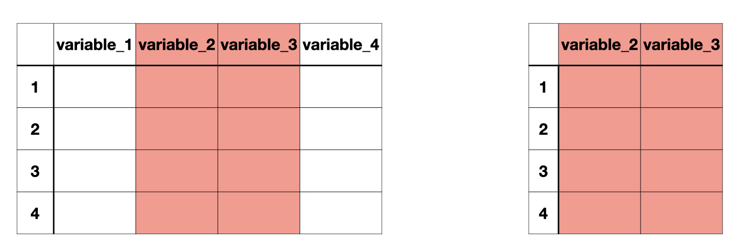
Column-wise subsetting can be done using select().

subsetting observations/rows

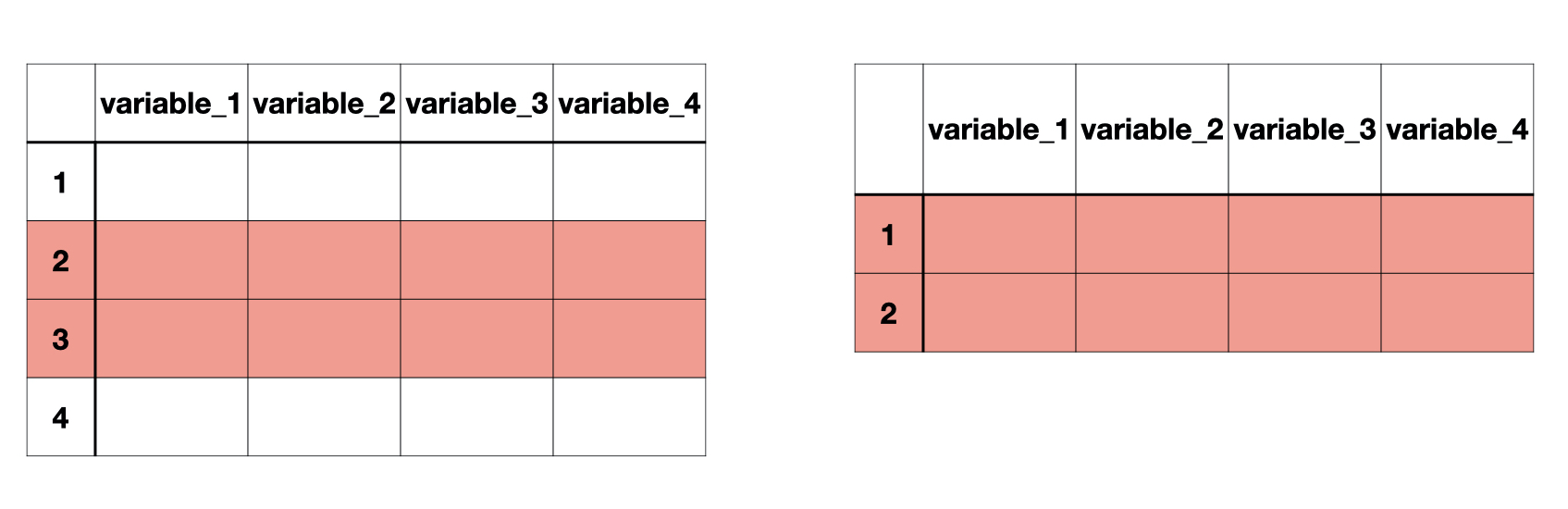
. . . Row-wise subsetting can be done with slice() and filter()

select is used to select certain variables in the data frame.

select(covid_data, pan_day, result)

# A tibble: 15,524 × 2
   pan_day result  
     <dbl> <chr>   
 1       4 negative
 2       7 negative
 3       7 negative
 4       8 negative
 5       8 negative
 6       8 negative
 7       9 negative
 8       9 negative
 9       9 negative
10       9 negative
# ℹ 15,514 more rows

covid_data |> 
  select(pan_day, result)

# A tibble: 15,524 × 2
   pan_day result  
     <dbl> <chr>   
 1       4 negative
 2       7 negative
 3       7 negative
 4       8 negative
 5       8 negative
 6       8 negative
 7       9 negative
 8       9 negative
 9       9 negative
10       9 negative
# ℹ 15,514 more rows

select can also be used to drop certain variables if used with a negative sign.

select(covid_data, -subject_id, -demo_group)

# A tibble: 15,524 × 15
   fake_first_name fake_last_name gender pan_day test_id clinic_name      result
   <chr>           <chr>          <chr>    <dbl> <chr>   <chr>            <chr> 
 1 jhezane         westerling     female       4 covid   inpatient ward a negat…
 2 penny           targaryen      female       7 covid   clinical lab     negat…
 3 grunt           rivers         male         7 covid   clinical lab     negat…
 4 melisandre      swyft          female       8 covid   clinical lab     negat…
 5 rolley          karstark       male         8 covid   emergency dept   negat…
 6 megga           karstark       female       8 covid   oncology day ho… negat…
 7 ithoke          targaryen      male         9 covid   clinical lab     negat…
 8 ravella         frey           female       9 covid   emergency dept   negat…
 9 styr            tyrell         male         9 covid   clinical lab     negat…
10 wynafryd        seaworth       male         9 covid   clinical lab     negat…
# ℹ 15,514 more rows
# ℹ 8 more variables: age <dbl>, drive_thru_ind <dbl>, ct_result <dbl>,
#   orderset <dbl>, payor_group <chr>, patient_class <chr>, col_rec_tat <dbl>,
#   rec_ver_tat <dbl>

Selection helpers

starts_with()
ends_with()
contains()

select(covid_data, starts_with("f"))

# A tibble: 15,524 × 2
   fake_first_name fake_last_name
   <chr>           <chr>         
 1 jhezane         westerling    
 2 penny           targaryen     
 3 grunt           rivers        
 4 melisandre      swyft         
 5 rolley          karstark      
 6 megga           karstark      
 7 ithoke          targaryen     
 8 ravella         frey          
 9 styr            tyrell        
10 wynafryd        seaworth      
# ℹ 15,514 more rows

select(covid_data, ends_with("name"))

# A tibble: 15,524 × 3
   fake_first_name fake_last_name clinic_name      
   <chr>           <chr>          <chr>            
 1 jhezane         westerling     inpatient ward a 
 2 penny           targaryen      clinical lab     
 3 grunt           rivers         clinical lab     
 4 melisandre      swyft          clinical lab     
 5 rolley          karstark       emergency dept   
 6 megga           karstark       oncology day hosp
 7 ithoke          targaryen      clinical lab     
 8 ravella         frey           emergency dept   
 9 styr            tyrell         clinical lab     
10 wynafryd        seaworth       clinical lab     
# ℹ 15,514 more rows

select(covid_data, contains("rec"))

# A tibble: 15,524 × 2
   col_rec_tat rec_ver_tat
         <dbl>       <dbl>
 1         1.4         5.2
 2         2.3         5.8
 3         7.3         4.7
 4         5.8         5  
 5         1.2         6.4
 6         1.4         7  
 7         2.6         4.2
 8         0.7         6.3
 9         1           5.6
10         7.1         7  
# ℹ 15,514 more rows

slice() subsets rows based on a row number.

The data below include all the rows from third to seventh, including the third and the seventh.

slice(covid_data, 3:7)

# A tibble: 5 × 17
  subject_id fake_first_name fake_last_name gender pan_day test_id clinic_name  
       <dbl> <chr>           <chr>          <chr>    <dbl> <chr>   <chr>        
1       9134 grunt           rivers         male         7 covid   clinical lab 
2       8518 melisandre      swyft          female       8 covid   clinical lab 
3       8967 rolley          karstark       male         8 covid   emergency de…
4      11048 megga           karstark       female       8 covid   oncology day…
5        663 ithoke          targaryen      male         9 covid   clinical lab 
# ℹ 10 more variables: result <chr>, demo_group <chr>, age <dbl>,
#   drive_thru_ind <dbl>, ct_result <dbl>, orderset <dbl>, payor_group <chr>,
#   patient_class <chr>, col_rec_tat <dbl>, rec_ver_tat <dbl>

Relational Operators in R

Operator	Description
<	Less than
>	Greater than
<=	Less than or equal to
>=	Greater than or equal to
==	Equal to
!=	Not equal to

Logical Operators in R

Operator	Description
&	and
|	or

filter() subsets rows based on a condition.

The data below includes rows when the clinic name is “emergency dept”

filter(covid_data, clinic_name == "emergency dept")

# A tibble: 3,413 × 17
   subject_id fake_first_name fake_last_name gender pan_day test_id clinic_name 
        <dbl> <chr>           <chr>          <chr>    <dbl> <chr>   <chr>       
 1       8967 rolley          karstark       male         8 covid   emergency d…
 2       2158 ravella         frey           female       9 covid   emergency d…
 3       4930 sarra           frey           female      10 covid   emergency d…
 4       2083 weasel          tarly          female      10 covid   emergency d…
 5      10468 chella          mormont        female      10 covid   emergency d…
 6        227 maege           sand           female      11 covid   emergency d…
 7       2983 ronnel          snow           male        11 covid   emergency d…
 8       6569 lanna           baelish        female      11 covid   emergency d…
 9       8165 arianne         clegane        female      11 covid   emergency d…
10       8395 nan             frey           female      11 covid   emergency d…
# ℹ 3,403 more rows
# ℹ 10 more variables: result <chr>, demo_group <chr>, age <dbl>,
#   drive_thru_ind <dbl>, ct_result <dbl>, orderset <dbl>, payor_group <chr>,
#   patient_class <chr>, col_rec_tat <dbl>, rec_ver_tat <dbl>

Q. How many tests performed in the emergency department were positive?

covid_data |> 
  filter(result == "positive" & clinic_name == "emergency dept")

# A tibble: 180 × 17
   subject_id fake_first_name fake_last_name gender pan_day test_id clinic_name 
        <dbl> <chr>           <chr>          <chr>    <dbl> <chr>   <chr>       
 1        902 owen            seaworth       male        12 covid   emergency d…
 2       2573 glendon         lannister      male        12 covid   emergency d…
 3      10734 jyck            sand           male        12 covid   emergency d…
 4       5023 chataya         mormont        female      15 covid   emergency d…
 5       6493 sybelle         karstark       female      16 covid   emergency d…
 6       8662 ronald          manderly       male        16 covid   emergency d…
 7       8685 black           lannister      male        16 covid   emergency d…
 8      11411 alysane         baelish        female      16 covid   emergency d…
 9       1131 ermesande       clegane        female      18 covid   emergency d…
10       7953 anya            westerling     female      18 covid   emergency d…
# ℹ 170 more rows
# ℹ 10 more variables: result <chr>, demo_group <chr>, age <dbl>,
#   drive_thru_ind <dbl>, ct_result <dbl>, orderset <dbl>, payor_group <chr>,
#   patient_class <chr>, col_rec_tat <dbl>, rec_ver_tat <dbl>

covid_data |> 
  filter(result == "positive" & clinic_name == "emergency dept") |> 
  nrow()

[1] 180

Q. How many observations are available between 10th and 50th day of the pandemic?

covid_data |> 
  filter(pan_day >= 10 & pan_day <= 50) 

# A tibble: 5,667 × 17
   subject_id fake_first_name fake_last_name gender pan_day test_id clinic_name 
        <dbl> <chr>           <chr>          <chr>    <dbl> <chr>   <chr>       
 1        998 harra           sand           female      10 covid   clinical lab
 2       2103 ollo            snow           male        10 covid   clinical lab
 3       2349 yezzan          royce          male        10 covid   line clinic…
 4       4930 sarra           frey           female      10 covid   emergency d…
 5       5408 alia            ryswell        female      10 covid   clinical lab
 6       2083 weasel          tarly          female      10 covid   emergency d…
 7       8031 gueren          sand           male        10 covid   clinical lab
 8       8138 frenya          swyft          female      10 covid   clinical lab
 9       9502 lorcas          mormont        male        10 covid   clinical lab
10      10468 chella          mormont        female      10 covid   emergency d…
# ℹ 5,657 more rows
# ℹ 10 more variables: result <chr>, demo_group <chr>, age <dbl>,
#   drive_thru_ind <dbl>, ct_result <dbl>, orderset <dbl>, payor_group <chr>,
#   patient_class <chr>, col_rec_tat <dbl>, rec_ver_tat <dbl>

covid_data |> 
  filter(pan_day >= 10 & pan_day <= 50) |>  
  nrow()

[1] 5667

Q. How many patients 18 years and older were tested in the emergency department?

covid_data |> 
  filter(age >= 18 & clinic_name <= "emergency dept") |>  
  nrow()

[1] 3337

We have done all sorts of selections, slicing, filtering on covid_data but it has not changed at all. Why do you think so?

glimpse(covid_data)

Rows: 15,524
Columns: 17
$ subject_id      <dbl> 1412, 533, 9134, 8518, 8967, 11048, 663, 2158, 3794, 4…
$ fake_first_name <chr> "jhezane", "penny", "grunt", "melisandre", "rolley", "…
$ fake_last_name  <chr> "westerling", "targaryen", "rivers", "swyft", "karstar…
$ gender          <chr> "female", "female", "male", "female", "male", "female"…
$ pan_day         <dbl> 4, 7, 7, 8, 8, 8, 9, 9, 9, 9, 9, 9, 9, 9, 9, 10, 10, 1…
$ test_id         <chr> "covid", "covid", "covid", "covid", "covid", "covid", …
$ clinic_name     <chr> "inpatient ward a", "clinical lab", "clinical lab", "c…
$ result          <chr> "negative", "negative", "negative", "negative", "negat…
$ demo_group      <chr> "patient", "patient", "patient", "patient", "patient",…
$ age             <dbl> 0.0, 0.0, 0.8, 0.8, 0.8, 0.8, 0.8, 0.0, 0.0, 0.9, 0.9,…
$ drive_thru_ind  <dbl> 0, 1, 1, 1, 0, 0, 1, 0, 1, 1, 1, 0, 0, 1, 1, 1, 1, 0, …
$ ct_result       <dbl> 45, 45, 45, 45, 45, 45, 45, 45, 45, 45, 45, 45, 45, 45…
$ orderset        <dbl> 0, 0, 1, 1, 1, 0, 1, 1, 1, 1, 0, 1, 0, 1, 1, 1, 1, 1, …
$ payor_group     <chr> "government", "commercial", NA, NA, "government", "com…
$ patient_class   <chr> "inpatient", "not applicable", NA, NA, "emergency", "r…
$ col_rec_tat     <dbl> 1.4, 2.3, 7.3, 5.8, 1.2, 1.4, 2.6, 0.7, 1.0, 7.1, 2.5,…
$ rec_ver_tat     <dbl> 5.2, 5.8, 4.7, 5.0, 6.4, 7.0, 4.2, 6.3, 5.6, 7.0, 3.8,…

If we want to create a smaller data frame, we can always save it in a new object:

covid_data_smaller <- 
  covid_data |> 
  filter(pan_day <= 10) |> 
  select(subject_id, 
         pan_day,
         result, 
         clinic_name)

glimpse(covid_data_smaller)

Rows: 28
Columns: 4
$ subject_id  <dbl> 1412, 533, 9134, 8518, 8967, 11048, 663, 2158, 3794, 4706,…
$ pan_day     <dbl> 4, 7, 7, 8, 8, 8, 9, 9, 9, 9, 9, 9, 9, 9, 9, 10, 10, 10, 1…
$ result      <chr> "negative", "negative", "negative", "negative", "negative"…
$ clinic_name <chr> "inpatient ward a", "clinical lab", "clinical lab", "clini…

Changing Variables

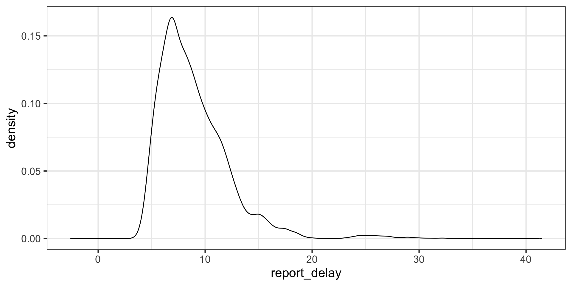
Goal:

Create a new variable called report_delay that represents the number of hours it took for the test result to be reported inside the clinical surveillance system.

covid_data |> 
  mutate(report_delay = col_rec_tat + rec_ver_tat)

# A tibble: 15,524 × 18
   subject_id fake_first_name fake_last_name gender pan_day test_id clinic_name 
        <dbl> <chr>           <chr>          <chr>    <dbl> <chr>   <chr>       
 1       1412 jhezane         westerling     female       4 covid   inpatient w…
 2        533 penny           targaryen      female       7 covid   clinical lab
 3       9134 grunt           rivers         male         7 covid   clinical lab
 4       8518 melisandre      swyft          female       8 covid   clinical lab
 5       8967 rolley          karstark       male         8 covid   emergency d…
 6      11048 megga           karstark       female       8 covid   oncology da…
 7        663 ithoke          targaryen      male         9 covid   clinical lab
 8       2158 ravella         frey           female       9 covid   emergency d…
 9       3794 styr            tyrell         male         9 covid   clinical lab
10       4706 wynafryd        seaworth       male         9 covid   clinical lab
# ℹ 15,514 more rows
# ℹ 11 more variables: result <chr>, demo_group <chr>, age <dbl>,
#   drive_thru_ind <dbl>, ct_result <dbl>, orderset <dbl>, payor_group <chr>,
#   patient_class <chr>, col_rec_tat <dbl>, rec_ver_tat <dbl>,
#   report_delay <dbl>

We can use pipes with ggplot too!

covid_data |> 
  mutate(report_delay = col_rec_tat + rec_ver_tat) |> 
  ggplot(aes(x = report_delay)) +
  geom_density() + 
  theme_bw(base_size = 16)

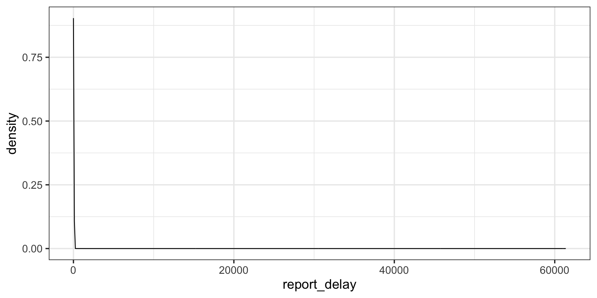
What is going on here? Maybe we have lots of outliers?

covid_data |> 
  mutate(report_delay = col_rec_tat + rec_ver_tat) |>
  filter(report_delay > 240) # longer than 10 days

# A tibble: 7 × 18
  subject_id fake_first_name fake_last_name gender pan_day test_id clinic_name  
       <dbl> <chr>           <chr>          <chr>    <dbl> <chr>   <chr>        
1       5018 shirei          royce          female      41 covid   inpatient wa…
2       2193 wilbert         sand           male        45 covid   inpatient wa…
3       4860 selyse          manderly       female      46 covid   line clinica…
4        801 tanda           westerling     female      56 covid   1 laboratory 
5        214 rowan           harlaw         male        79 covid   autopsy      
6       1306 dick            clegane        male        84 covid   inpatient wa…
7      11684 anguy           stark          male        95 covid   autopsy      
# ℹ 11 more variables: result <chr>, demo_group <chr>, age <dbl>,
#   drive_thru_ind <dbl>, ct_result <dbl>, orderset <dbl>, payor_group <chr>,
#   patient_class <chr>, col_rec_tat <dbl>, rec_ver_tat <dbl>,
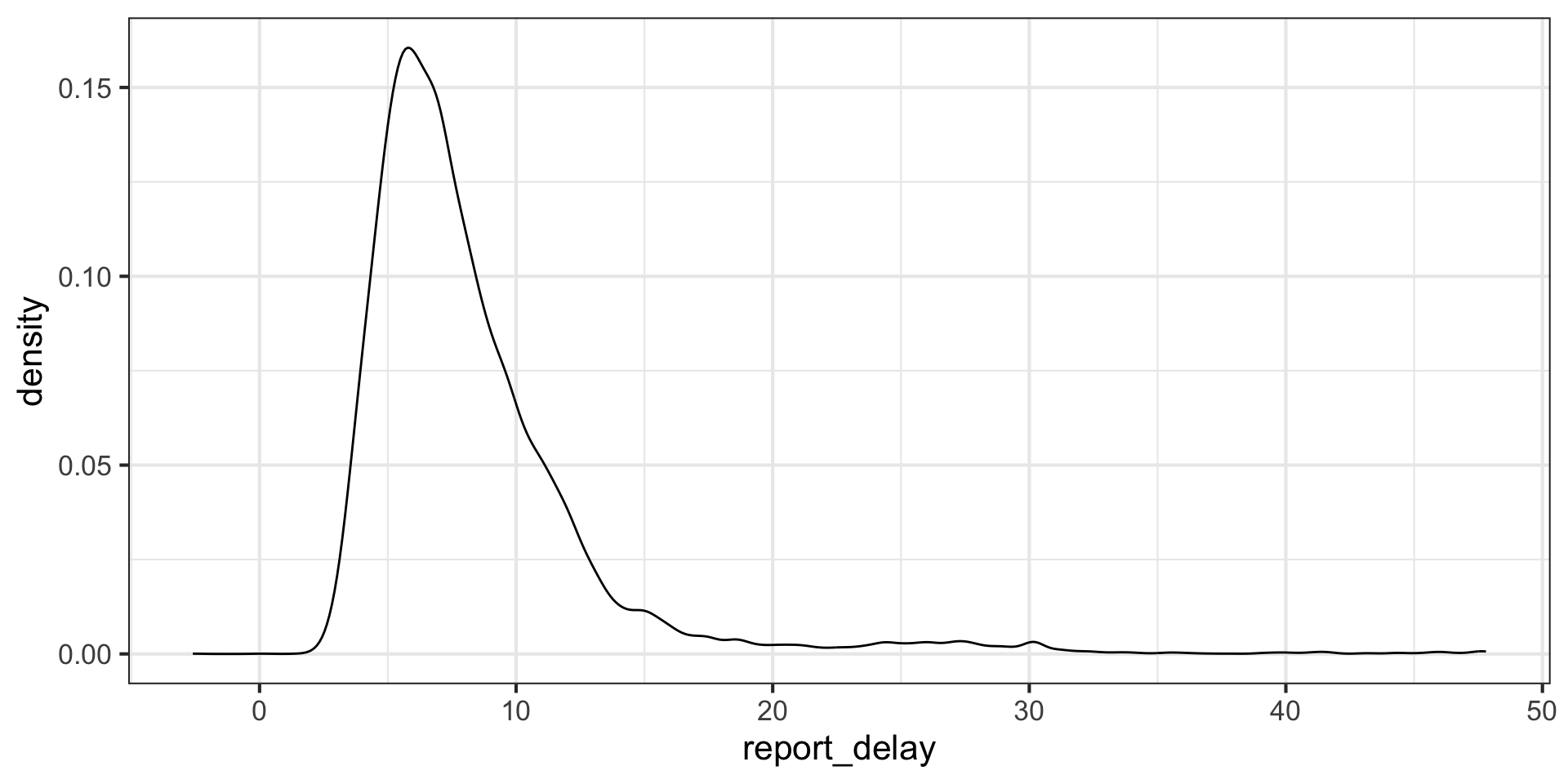
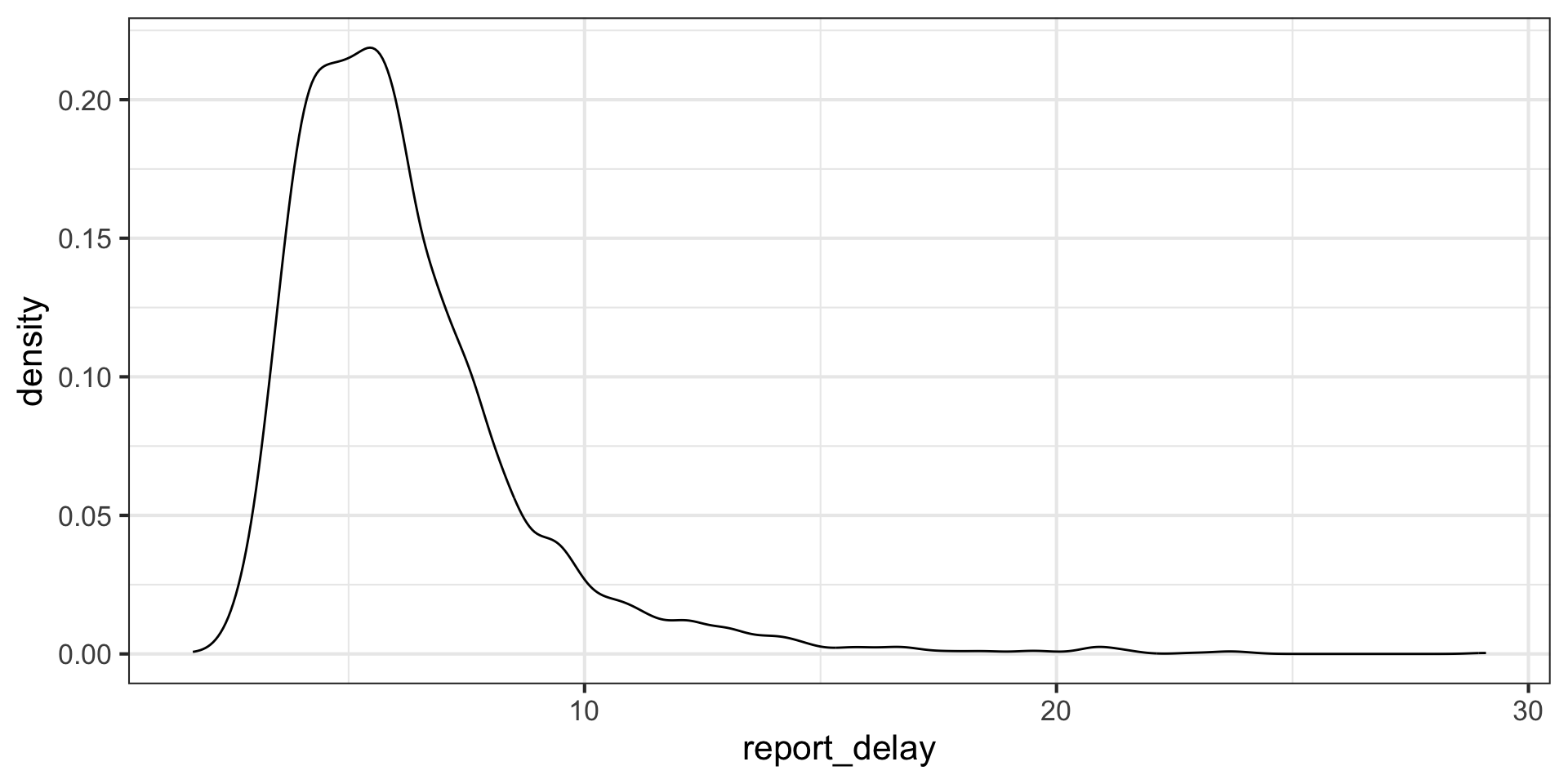
#   report_delay <dbl>

Let’s look at the distribution of reporting delays filtering them to be below 48 hours:

covid_data |> 
  mutate(report_delay = col_rec_tat + rec_ver_tat) |> 
  filter(report_delay < 48) |>
  ggplot(aes(x = report_delay)) +
  geom_density() +
  theme_bw(base_size = 16)

covid_data |> 
  mutate(report_delay = col_rec_tat + rec_ver_tat) |> 
  group_by(pan_day) |>
  summarize(num_positive_tests = sum(result=="positive"), num_negative_tests = sum(result=="negative"), total_tests=n())

# A tibble: 102 × 4
   pan_day num_positive_tests num_negative_tests total_tests
     <dbl>              <int>              <int>       <int>
 1       4                  0                  1           1
 2       7                  0                  2           2
 3       8                  0                  3           3
 4       9                  0                  9           9
 5      10                  1                 12          13
 6      11                  2                 69          71
 7      12                  4                 44          48
 8      13                  3                 28          31
 9      14                  2                 45          47
10      15                  1                 46          50
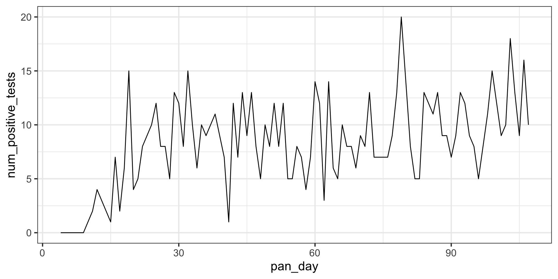
# ℹ 92 more rows

Let’s look at the positive tests as a function of time

covid_data |> 
  mutate(report_delay = col_rec_tat + rec_ver_tat) |> 
  group_by(pan_day) |>
  summarize(num_positive_tests = sum(result=="positive"), num_negative_tests = sum(result=="negative"), total_tests=n()) |> 
  ggplot(aes(x = pan_day, y = num_positive_tests)) +
  geom_line() +
  theme_bw(base_size = 16)

Your task:

• Investigate differences in reporting delays between emergency department and clinic lab tests

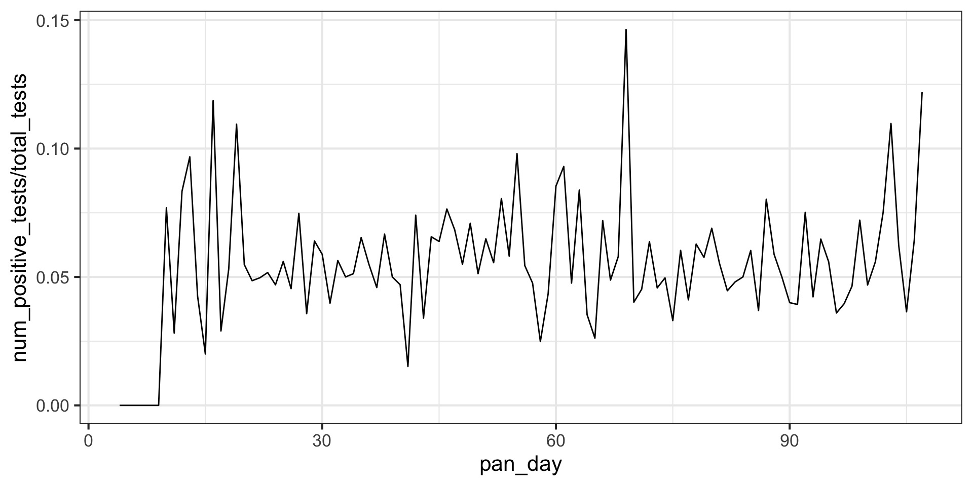
• Plot test positivity (number of positive tests divided by the number of negative tests) as a function of time. What differences do you see between this time series and the time series of positive tests?

Task 1 solution:

covid_data |> 
  mutate(report_delay = col_rec_tat + rec_ver_tat) |> 
  filter(report_delay < 48 & clinic_name == "emergency dept") |>
  ggplot(aes(x = report_delay)) +
  geom_density() +
  theme_bw(base_size = 16)

covid_data |> 
  mutate(report_delay = col_rec_tat + rec_ver_tat) |> 
  filter(report_delay < 48 & clinic_name == "clinical lab") |>
  ggplot(aes(x = report_delay)) +
  geom_density() +
  theme_bw(base_size = 16)

Task 2 solution:

covid_data |> 
  mutate(report_delay = col_rec_tat + rec_ver_tat) |> 
  group_by(pan_day) |>
  summarize(num_positive_tests = sum(result=="positive"), num_negative_tests = sum(result=="negative"), total_tests=n()) |> 
  ggplot(aes(x = pan_day, y = num_positive_tests/total_tests)) +
  geom_line() +
  theme_bw(base_size = 16)