Data Wrangling
Part II

ISI-BUDS 2025

Data

library(medicaldata)
covid_data <- medicaldata::covid_testing
glimpse(covid_data)

Rows: 15,524
Columns: 17
$ subject_id      <dbl> 1412, 533, 9134, 8518, 8967, 11048, 663, 2158, 3794, 4…
$ fake_first_name <chr> "jhezane", "penny", "grunt", "melisandre", "rolley", "…
$ fake_last_name  <chr> "westerling", "targaryen", "rivers", "swyft", "karstar…
$ gender          <chr> "female", "female", "male", "female", "male", "female"…
$ pan_day         <dbl> 4, 7, 7, 8, 8, 8, 9, 9, 9, 9, 9, 9, 9, 9, 9, 10, 10, 1…
$ test_id         <chr> "covid", "covid", "covid", "covid", "covid", "covid", …
$ clinic_name     <chr> "inpatient ward a", "clinical lab", "clinical lab", "c…
$ result          <chr> "negative", "negative", "negative", "negative", "negat…
$ demo_group      <chr> "patient", "patient", "patient", "patient", "patient",…
$ age             <dbl> 0.0, 0.0, 0.8, 0.8, 0.8, 0.8, 0.8, 0.0, 0.0, 0.9, 0.9,…
$ drive_thru_ind  <dbl> 0, 1, 1, 1, 0, 0, 1, 0, 1, 1, 1, 0, 0, 1, 1, 1, 1, 0, …
$ ct_result       <dbl> 45, 45, 45, 45, 45, 45, 45, 45, 45, 45, 45, 45, 45, 45…
$ orderset        <dbl> 0, 0, 1, 1, 1, 0, 1, 1, 1, 1, 0, 1, 0, 1, 1, 1, 1, 1, …
$ payor_group     <chr> "government", "commercial", NA, NA, "government", "com…
$ patient_class   <chr> "inpatient", "not applicable", NA, NA, "emergency", "r…
$ col_rec_tat     <dbl> 1.4, 2.3, 7.3, 5.8, 1.2, 1.4, 2.6, 0.7, 1.0, 7.1, 2.5,…
$ rec_ver_tat     <dbl> 5.2, 5.8, 4.7, 5.0, 6.4, 7.0, 4.2, 6.3, 5.6, 7.0, 3.8,…

Aggregating Data

Data

Observations

Aggregate Data

Summaries of observations

Aggregating Categorical Data

Categorical data are summarized with counts or proportions.

covid_data |> 
  count(result)

# A tibble: 3 × 2
  result       n
  <chr>    <int>
1 invalid    301
2 negative 14358
3 positive   865

covid_data |> 
  count(result) |> 
  mutate(prop = n/sum(n))

# A tibble: 3 × 3
  result       n   prop
  <chr>    <int>  <dbl>
1 invalid    301 0.0194
2 negative 14358 0.925 
3 positive   865 0.0557

Aggregating Numerical Data

Mean, median, standard deviation, variance, and quartiles are some of the numerical summaries of numerical variables.

covid_data |> 
  mutate(report_delay = col_rec_tat + rec_ver_tat) |> 
  filter(report_delay <= 48) |> 
  summarize(mean_report_delay = mean(report_delay),
          sd_report_delay = sd(report_delay))

# A tibble: 1 × 2
  mean_report_delay sd_report_delay
              <dbl>           <dbl>
1              8.36            4.84

Aggregating Data By Groups

`group_by()`

We have used this function yesterday to aggregate data into daily counts of test results. Let’s review and use this function for other types of groups.

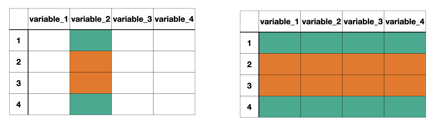
group_by() separates the data frame by the groups. Any action following group_by() will be completed for each group separately.

Q. What is the median test reporting delay for each clinic type?

covid_data |> 
  group_by(clinic_name)

# A tibble: 15,524 × 17
# Groups:   clinic_name [88]
   subject_id fake_first_name fake_last_name gender pan_day test_id clinic_name 
        <dbl> <chr>           <chr>          <chr>    <dbl> <chr>   <chr>       
 1       1412 jhezane         westerling     female       4 covid   inpatient w…
 2        533 penny           targaryen      female       7 covid   clinical lab
 3       9134 grunt           rivers         male         7 covid   clinical lab
 4       8518 melisandre      swyft          female       8 covid   clinical lab
 5       8967 rolley          karstark       male         8 covid   emergency d…
 6      11048 megga           karstark       female       8 covid   oncology da…
 7        663 ithoke          targaryen      male         9 covid   clinical lab
 8       2158 ravella         frey           female       9 covid   emergency d…
 9       3794 styr            tyrell         male         9 covid   clinical lab
10       4706 wynafryd        seaworth       male         9 covid   clinical lab
# ℹ 15,514 more rows
# ℹ 10 more variables: result <chr>, demo_group <chr>, age <dbl>,
#   drive_thru_ind <dbl>, ct_result <dbl>, orderset <dbl>, payor_group <chr>,
#   patient_class <chr>, col_rec_tat <dbl>, rec_ver_tat <dbl>

Note that when group_by() is used there have been no changes to the number of columns or rows. The only difference we can observe is now Groups: clinic_name [88] is displayed indicating the data frame (i.e., tibble) is divided into three groups.

covid_data |> 
  group_by(clinic_name) |> 
  mutate(report_delay = col_rec_tat + rec_ver_tat) |> 
  filter(report_delay <= 48) |>
  summarize(med_report_delay = median(report_delay))

# A tibble: 88 × 2
   clinic_name           med_report_delay
   <chr>                            <dbl>
 1 1 laboratory                      8.7 
 2 3  laboratory                     7.05
 3 anes resource ctr                 5.8 
 4 apheresis                         7.1 
 5 autopsy                           6.7 
 6 bed management center            29.6 
 7 behavioral hosp                   9.15
 8 bmc                              15.7 
 9 cardiac echo                      5.6 
10 cardiac ekg                       5   
# ℹ 78 more rows

We can also remind ourselves how many tests were performed in each clinic group.

covid_data |> 
  group_by(clinic_name) |> 
  mutate(report_delay = col_rec_tat + rec_ver_tat) |> 
  filter(report_delay <= 48) |>
  summarize(med_report_delay = median(report_delay), count=n())

# A tibble: 88 × 3
   clinic_name           med_report_delay count
   <chr>                            <dbl> <int>
 1 1 laboratory                      8.7      2
 2 3  laboratory                     7.05     2
 3 anes resource ctr                 5.8      3
 4 apheresis                         7.1      1
 5 autopsy                           6.7      7
 6 bed management center            29.6      1
 7 behavioral hosp                   9.15    98
 8 bmc                              15.7      1
 9 cardiac echo                      5.6      2
10 cardiac ekg                       5        7
# ℹ 78 more rows

Note that n() does not take any arguments.

Data Joins

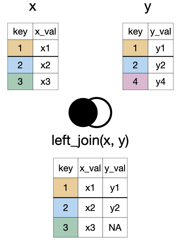
`left_join(x, y)`

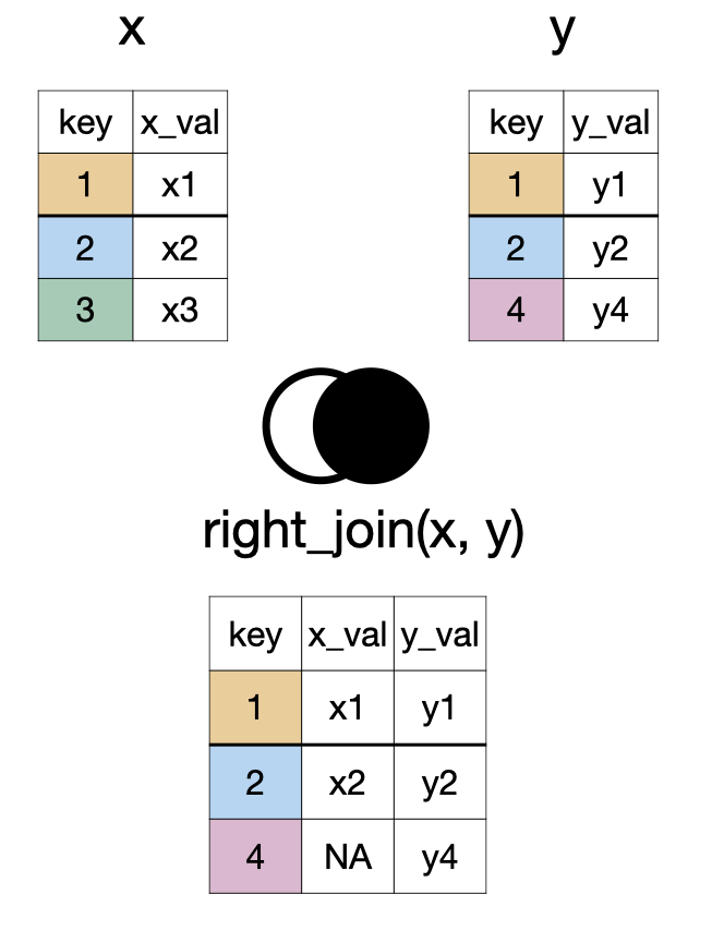
`right_join(x, y)`

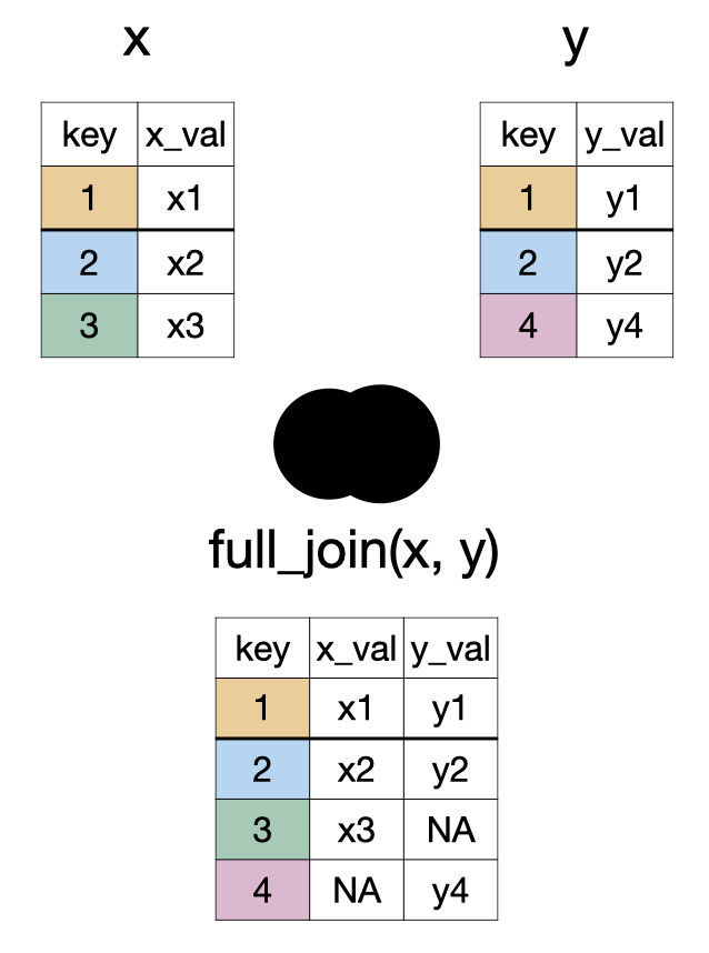
`full_join(x, y)`

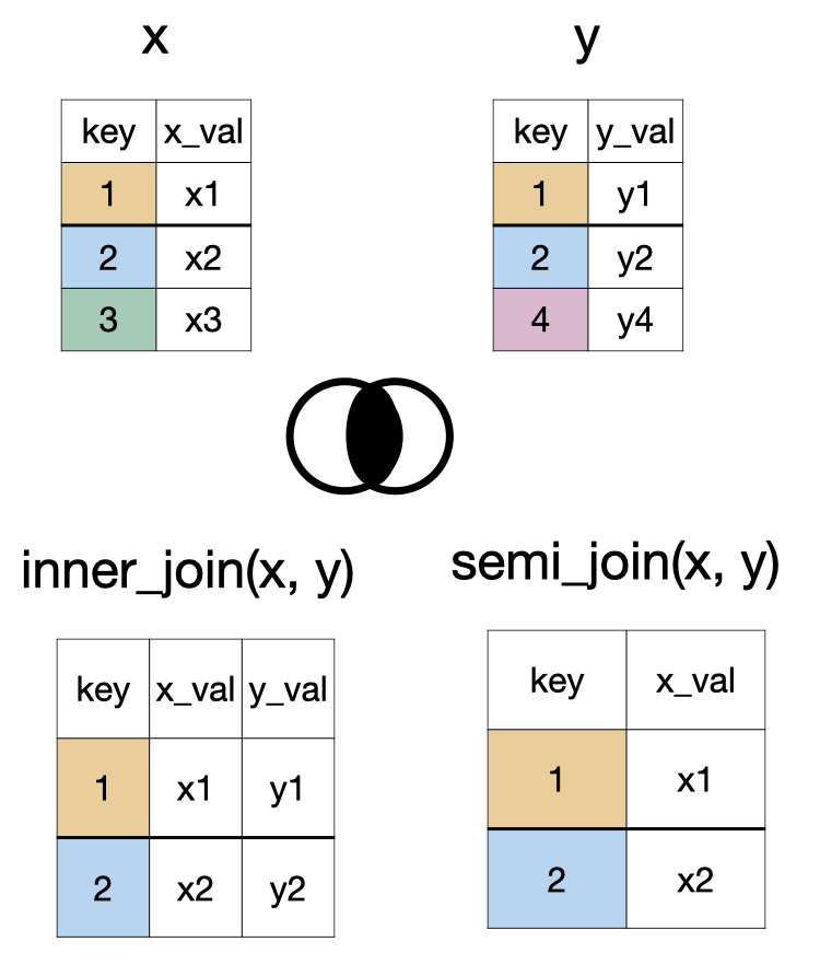
`inner_join(x, y)` and `semi_join(x, y)`

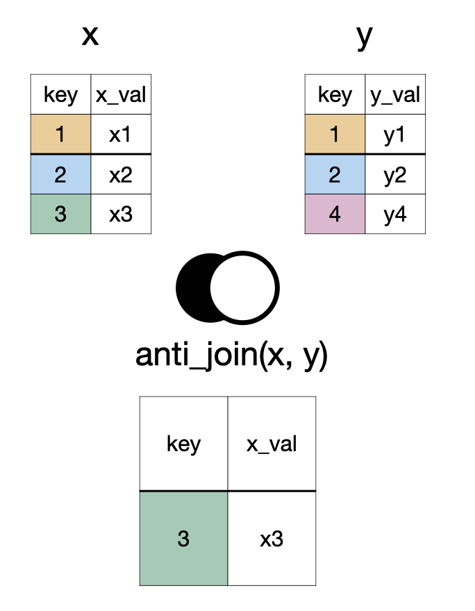
`anti_join(x, y)`

`something_join(x, y)`

	x		y
	rows	columns	rows	columns
`left_join()`	all	all	matched	all
`right_join()`	matched	all	all	all
`full_join()`	all	all	all	all
`inner_join()`	matched	all	matched	all
`semi_join()`	matched	all	none	none
`anti_join()`	unmatched	all	none	none

artists
songs
albums

artists

# A tibble: 3 × 2
  name          followers
  <chr>             <dbl>
1 Beyoncé        24757958
2 Taylor Swift   33098116
3 Ariana Grande  51807131

songs

# A tibble: 5 × 4
  name          song_name                            album_name  song_popularity
  <chr>         <chr>                                <chr>                 <dbl>
1 Beyoncé       Savage Remix (feat. Beyoncé)         Savage Rem…              83
2 Taylor Swift  cardigan                             folklore                 85
3 Drake         Laugh Now Cry Later (feat. Lil Durk) Laugh Now …              95
4 Beyoncé       Halo                                 I AM…SASHA…              NA
5 Ariana Grande Stuck with U (with Justin Bieber)    Stuck with…              NA

albums

# A tibble: 4 × 2
  album_name                           album_release_date
  <chr>                                <date>            
1 Savage Remix (feat. Beyoncé)         2020-04-29        
2 I AM…SASHA FIERCE                    2008-11-14        
3 Stuck with U                         2020-05-08        
4 Laugh Now Cry Later (feat. Lil Durk) 2020-08-14

left_join(songs, artists)

# A tibble: 5 × 5
  name          song_name                   album_name song_popularity followers
  <chr>         <chr>                       <chr>                <dbl>     <dbl>
1 Beyoncé       Savage Remix (feat. Beyonc… Savage Re…              83  24757958
2 Taylor Swift  cardigan                    folklore                85  33098116
3 Drake         Laugh Now Cry Later (feat.… Laugh Now…              95        NA
4 Beyoncé       Halo                        I AM…SASH…              NA  24757958
5 Ariana Grande Stuck with U (with Justin … Stuck wit…              NA  51807131

right_join(songs, artists)

# A tibble: 4 × 5
  name          song_name                   album_name song_popularity followers
  <chr>         <chr>                       <chr>                <dbl>     <dbl>
1 Beyoncé       Savage Remix (feat. Beyonc… Savage Re…              83  24757958
2 Taylor Swift  cardigan                    folklore                85  33098116
3 Beyoncé       Halo                        I AM…SASH…              NA  24757958
4 Ariana Grande Stuck with U (with Justin … Stuck wit…              NA  51807131

full_join(songs, artists, by = "name")

# A tibble: 5 × 5
  name          song_name                   album_name song_popularity followers
  <chr>         <chr>                       <chr>                <dbl>     <dbl>
1 Beyoncé       Savage Remix (feat. Beyonc… Savage Re…              83  24757958
2 Taylor Swift  cardigan                    folklore                85  33098116
3 Drake         Laugh Now Cry Later (feat.… Laugh Now…              95        NA
4 Beyoncé       Halo                        I AM…SASH…              NA  24757958
5 Ariana Grande Stuck with U (with Justin … Stuck wit…              NA  51807131

full_join(songs, artists, by = "name") |> 
  full_join(albums, by = "album_name")

# A tibble: 5 × 6
  name         song_name album_name song_popularity followers album_release_date
  <chr>        <chr>     <chr>                <dbl>     <dbl> <date>            
1 Beyoncé      Savage R… Savage Re…              83  24757958 2020-04-29        
2 Taylor Swift cardigan  folklore                85  33098116 NA                
3 Drake        Laugh No… Laugh Now…              95        NA 2020-08-14        
4 Beyoncé      Halo      I AM…SASH…              NA  24757958 2008-11-14        
5 Ariana Gran… Stuck wi… Stuck wit…              NA  51807131 2020-05-08

Your tasks:

Download hospitalization data from CA Open Data Portal.
Load the data into R/RStudio using read_csv() function and compute average number of hospital beds for each county in California over the whole time span of the data. Use hospitalized confirmed COVID patients as your variable of interest.

Your tasks:

Download a file with county population sizes from Slack.
Load the data into R/RStudio using read_csv() function, join this table with the hospitalization data to plot a scatter plot of county averages of hospitalized COVID patients and county population sizes.
Compute county average hospitalized patients per 100,000 people

ca_covid_hosp <- read_csv("../data/ca_covid_hosp.csv") 
ca_county_pop <- read_csv("../data/county_pop.csv")

ca_average_covid_hosp <- ca_covid_hosp |> 
  group_by(county) |> 
  summarize(average_hosp_covid_patients = mean(hospitalized_covid_confirmed_patients, na.rm=TRUE)) 

ca_average_covid_hosp

# A tibble: 56 × 2
   county       average_hosp_covid_patients
   <chr>                              <dbl>
 1 Alameda                          106.   
 2 Amador                             3.10 
 3 Butte                             21.0  
 4 Calaveras                          1.11 
 5 Colusa                             1.67 
 6 Contra Costa                      65.7  
 7 Del Norte                          1.87 
 8 El Dorado                          6.04 
 9 Fresno                           139.   
10 Glenn                              0.899
# ℹ 46 more rows

ca_average_covid_hosp <- inner_join(ca_average_covid_hosp, ca_county_pop, by = "county") 

ca_average_covid_hosp

# A tibble: 56 × 3
   county       average_hosp_covid_patients pop_size
   <chr>                              <dbl>    <dbl>
 1 Alameda                          106.     1671329
 2 Amador                             3.10     39752
 3 Butte                             21.0     219186
 4 Calaveras                          1.11     45905
 5 Colusa                             1.67     21547
 6 Contra Costa                      65.7    1153526
 7 Del Norte                          1.87     27812
 8 El Dorado                          6.04    192843
 9 Fresno                           139.      999101
10 Glenn                              0.899    28393
# ℹ 46 more rows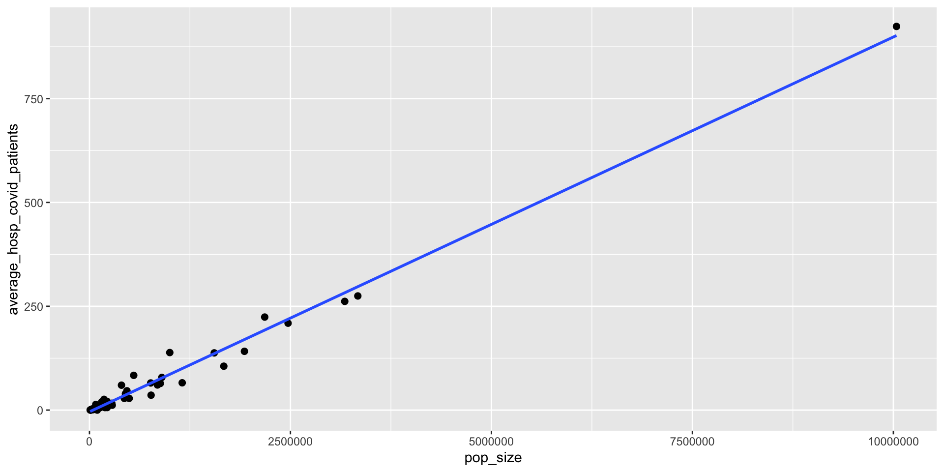

ca_average_covid_hosp |> 
  ggplot(aes(x=pop_size, y=average_hosp_covid_patients)) + 
  geom_point(size=2) + 
  geom_smooth(method=lm, se=FALSE)

ca_average_covid_hosp |>
  mutate(average_hosp_covid_patients_per_100K = average_hosp_covid_patients/pop_size*100000)

# A tibble: 56 × 4
   county       average_hosp_covid_patients pop_size average_hosp_covid_patien…¹
   <chr>                              <dbl>    <dbl>                       <dbl>
 1 Alameda                          106.     1671329                        6.33
 2 Amador                             3.10     39752                        7.79
 3 Butte                             21.0     219186                        9.57
 4 Calaveras                          1.11     45905                        2.41
 5 Colusa                             1.67     21547                        7.75
 6 Contra Costa                      65.7    1153526                        5.70
 7 Del Norte                          1.87     27812                        6.72
 8 El Dorado                          6.04    192843                        3.13
 9 Fresno                           139.      999101                       13.9 
10 Glenn                              0.899    28393                        3.17
# ℹ 46 more rows
# ℹ abbreviated name: ¹average_hosp_covid_patients_per_100K

Data Wrangling Part II

Data

Aggregating Data

Data

Aggregate Data

Aggregating Categorical Data

Aggregating Numerical Data

Aggregating Data By Groups

group_by()

Data Joins

left_join(x, y)

right_join(x, y)

full_join(x, y)

inner_join(x, y) and semi_join(x, y)

anti_join(x, y)

something_join(x, y)

Data Wrangling
Part II

`group_by()`

`left_join(x, y)`

`right_join(x, y)`

`full_join(x, y)`

`inner_join(x, y)` and `semi_join(x, y)`

`anti_join(x, y)`

`something_join(x, y)`